How To Change Legend Name In Excel Bar Chart

Select the Pivot Chart that you want to change its axis and legends and then show Filed List pane with clicking the Filed List button on the Analyze tab. I had originally answered with the following.

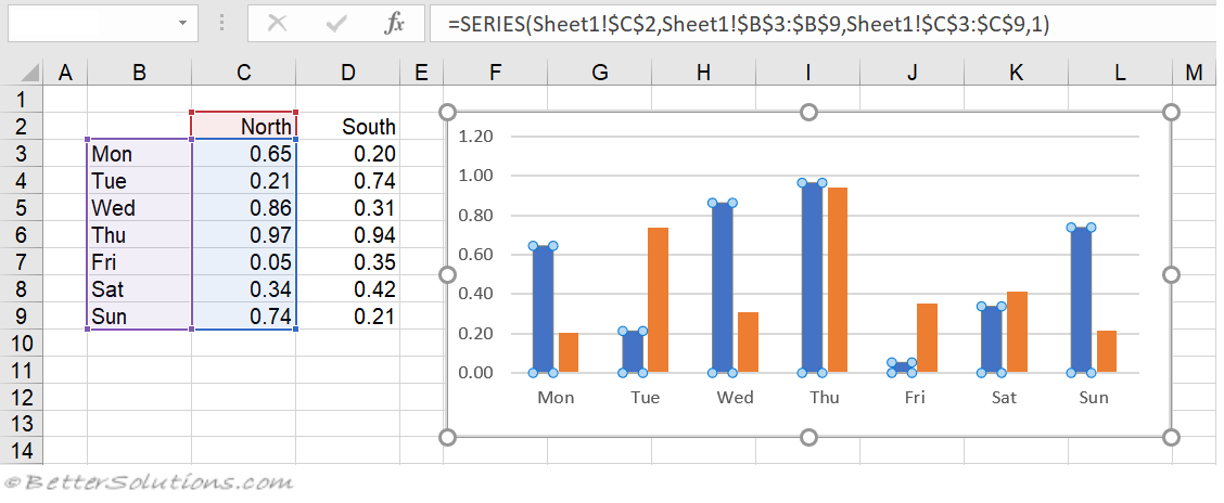
How To Rename Data Series In Excel Graph Or Chart Microsoft Excel Excel Data

Enter a new name into the Series Name or Name box.

How to change legend name in excel bar chart. I created a scatter plot graph that has 3 colored scatter plots on them. In the Select Data Source pop up under the Legend Entries section select the item to be reallocated and using the up or down arrow on. Click the legend then click the top legend label and hit the Delete key.

How To Make A Pie Chart In Excel Contextures. The following line of code is adding your unwanted Series2. Click Select Data on the toolbar.

You can change the Chart Title Axis titles of horizontal and vertical axis display values as labels display v. To rename a legend in a chart you can simply rewrite the data stored in the table that was used to create the graph. If you want to remove the chart title completely select your chart and click the Chart Elements icon on the right shown visually as a green symbol.

How To Change Legend Name In Excel Bar Chart. Learn how to change the elements of a chart. Note that SpreadsheetGear does use zero based indexes so chartSeriesCollection0 in SpreadsheetGear would be chartSeriesCollection1 in Excel or maybe chartSeriesCollectionItem1 since indexers dont always work as expected when using Excel via COM Interop.

How To Change Legend On A Pie Chart In Excel. Open a spreadsheet and click the chart you want to edit. Type a legend name into the Series name text box and click OK.

Gridlines in numbers on change legend names how to make a pie chart in microsoft excel how to create a pie chart in excel how to make a pie chart in excel. Your multiple data series will be listed under the Legend Entries Series column. Under the Data section click Select Data.

Today were gonna talk about the way to change the legend name. I right clicked on the legend and selected Format Legend. To change the text in the chart legend do the following.

Click the Design or Chart Design tab. If you really wanted to edit Series2 in the legend you would change it the same manner you changed the name of Series1. I tried clicking on the actual legend to try to change its name but it wont let me change the legend names.

The Easiest Way How to Rename a Legend in an Excel Chart. Youll then be able to edit or format the text as required. Click on the legend name you want to change in the Select Data Source dialog box and click Edit.

Select your chart in Excel and click Design Select Data. SeriesCollection 2Name Unwanted series. If the legend now has lots of white space select it and drag the legend corner points reduce its.

Legends In Chart How To Add And Remove Excel. And theres more than one. Posted on February 25 2021 by Eva.

To begin renaming your data series select. To reorder the bars click on the chart and select Chart Tools. Right-click the legend and choose Select Data in the context menu.

This will open the Select Data Source options window. The legend named it itself Series 1 Series 2 Series 3. The legend name in the chart changes to the new.

Posted on April 22 2021 by Eva. Automatically Legend names are created from contents of a cell on top of the row. To rename in excel graph chart and edit the legend in google sheets how to edit a legend in excel custom to rename a in microsoft excel remove legends in excel chart.

Be careful not to select the legends color box for the entry because then youll delete the data series. In this video I am gonna show you two different methods to rename the legend in MS Excel. In the Select Data Source dialog box under Legend Entries Series select the legend entry that you want to change and click the Edit button which resides above the list of the legend entries.

By default the Field List pane will be opened when clicking the pivot chart. To change the title text for a bar chart double-click the title text box above the chart itself. Enter a new value into the Y values box.

I will also show you how to put different marker signs in the lege. Select a legend entry and click Edit. To do this right-click your graph or chart and click the Select Data option.

Questions like how to edit legend in Excel how to change legend in Excel and how to edit legend in Excel has been asked so many times here are some few tips to help. So heres the first one the easiest way.

What Is Another Name For A Bar Chart

The may be shown using vertical or horizontal bars. A bar chart is a type of graph that is used to show and compare different measures for different categories of data or data series.

Pin By Gricelda Castellanoz On Theory Questions Specialty Class This Or That Questions Study Guide Bar Chart

The stacked bar chart aka stacked bar graph extends the standard bar chart from looking at numeric values across one categorical variable to two.

What is another name for a bar chart. A stacked bar chart is a bar chart that places related values atop one another. The labels tell us what kinds of facts are listed. A histogram is an example of a bar graph used in.

The bars show the facts. Use bar charts to compare data across categories. Ad Register Domain Name Free - This Is What Youre Searching For.

It is a common chart type with several price action strategies based on it. Each part of a bar graph has a purpose. The less editorialized your captions are the more credible your chart will seem.

The bars can be plotted vertically or horizontally. Rogets 21st Century Thesaurus Third Edition Copyright 2013 by the Philip Lief Group. A bar chart also known as a bar graph shows the differences between categories or trends over time using the length or height of its bars.

A type of vertical bar chart in which the categories are plotted in the descending rank order of the magnitude of their frequencies is called a. This chart type can either be in horizontal or in vertical orientation. Another name for a bar graph is a bar chart.

If there are any negative values they are stacked in reverse order below the charts axis baseline. Bar graphs are commonly used in financial analysis for displaying data. Stacked bar charts are typically used when a category naturally divides into components.

Lets deconstruct the definition by understanding components of a bar chart. One axis shows categories while the other a range of values. This chart is the first icon listed under the 2-D Column section.

A comparison graph is another name for a line chart. In vertical form it is usually called a column chart while in. There are a number of versions available so you can experiment with which option looks best.

See the Bar charts and types of data section below for more detail. Levels are plotted on one chart axis and values are plotted on the other axis. A bar chart aka bar graph column chart plots numeric values for levels of a categorical feature as bars.

Tableau selects this mark type when the data view matches one. Bar graphs are the pictorial representation of data generally grouped in the form of vertical or horizontal rectangular bars where the length of bars are proportional to the measure of data. We will learn how to create a bar chart in SAS Programming Language and the different types of SAS bar charts.

A vertical bar chart is sometimes called a column chart. A bar chart or bar graph is a chart or graph that presents categorical data with rectangular bars with heights or lengths proportional to the values that they represent. They are also known as bar charts.

So lets start the tutorial. What is Bar Chart in SAS. The important thing to know is that the longer the bar the greater its value.

For example here are two titles. A bar graph also known as a bar chart or bar diagram is a visual tool that uses bars to compare data among categories. An OHLC chart is a type of bar chart that shows open high low and closing prices.

Bar graphs have two axes. Some of the most common types of data charts include. A Pareto chart is a special example of a bar chart.

Bar graphs are one of the means of data handling in statistics. The title tells us what the graph is about. A Bar Graph also called Bar Chart is a graphical display of data using bars of different heights.

What is the difference between bar charts and Pareto charts. Grid lines are used to create the scale. A stock volume chart is a commonly used type of vertical bar graph.

The Massive Daily Revenue We Pulled in September 2015 Our Most Amazing Month. Stacked bar charts. Each categorical value claims one bar and the length of each bar corresponds to the bars value.

Bar charts are used with categorical or nominal data. You create a bar chart by placing a dimension on the Rows shelf and a measure on the Columns shelf or vice versa. For a Pareto chart the bars are ordered from highest to lowest.

Various column charts are available but to insert a standard bar chart click the Clustered Chart option. Excel will automatically take the data from your data set to create the chart on the same worksheet using your column labels to set axis and chart titles. Histograms are used with continuous data.

A bar graph may run horizontally or vertically. Creating a comparison graph is identical to creating a bar chart except you choose Line instead of Bar or Column. Each bar in a standard bar chart is divided into a number of sub-bars stacked end to end each one corresponding to.

SAS simple bar chart SAS stacked bar chart SAS grouped bar chart and SAS cluster bar chart SAS bar chart side by side. A bar chart uses the Bar mark type. Daily Revenue September 2015 If your revenue was massive it will show in the chart see the area chart above.

A bar chart also known as bar graph or bar diagram is a graphical representation of categorical data that presents and compares dependent and independent variables plotted along X-axis and Y-axis in form of rectangular bars. Synonyms for bar chart.

How To Display Series Name In Excel Chart

Change the Chart Type for the Average series to a Line chart. Select the series Brand A and click Edit.

Excel Charts Series Formula

I believe this may resolve your problem.

How to display series name in excel chart. 1 Select cells A2B5. The currently displayed source data is. 3 Select the desired Column type graph.

Edit Series preview pane. Then plot each point as its own series. In the Format Data Series pane under Fill Line tab click Line to display the Line section then check No line option.

Excel then adds these as new columns representing the data series. Just click on the map then choose from the Chart Design or Format tabs in the ribbon. The popup window will show you the chart type for each data series.

Then right click on the line in the chart to select Format Data Series from the context menu. Click anywhere in the chart. Learn how to change the elements of a chart.

Note that the chart does not yet display the 2015 data series. You can change the Chart Title Axis titles of horizontal and vertical axis display values as labels display v. The Edit Series dialog box will pop-up.

Change legend name Change Series Name in Select Data. Click the axis title box on the chart and type the text. This will also expose the map chart specific Series options see below.

Click Select Data button on the Design tab to open the Select Data Source dialog box. Change legend text through Select Data. Right-click anywhere on the chart and click Select Data.

In this example we have a chart that shows 2013 and 2014 quarterly sales data and weve just added a new data series to the worksheet for 2015. SERIES In the case of a bubble chart there is one additional argument. SERIES You can also view the series data using the Select Data dialogReviews.

There are spaces for series name and Y values. Please click to highlight the specified data series you will rename and then click the Edit button. In Excel 2003 choose Options from the Tools menu and skip to 3.

Add titles and series labels Click on the chart to open the Chart Tools contextual tab then edit the Chart title by clicking on the Chart Title textbox. Right click the chart and choose Select Data from the pop-up menu or click Select Data on the ribbon. Then format data labels to display series name for each of.

Since you want the average to show up as a line instead of columns right click on the data series and select Change Series Chart Type. This Excel Trick will help you to DisplayShow Formulas in Excel without any issues. Type the new series label in the Series name.

5 Select Data Labels Outside End was selected below If you dont want the Values as the Labels you can click on. Right click the chart whose data series you will rename and click Select Data from the right-clicking menu. Similarly for more such tips tricks you can follow our Excel Ninja Training and become an expert in Excel.

You can also double-click the chart to launch the Format Object Task Pane which will appear on the right-hand side of the Excel window. 4 Click on the graph to make sure it is selected then select Layout. I have a series of charts I am creating using VBA code below.

Click the File tab and choose Options. Changes over days or weeks andor the order of categories is not important. To edit the series labels follow these steps.

Another convoluted answer which should technically work and is ok for a small number of data points is to plot all your data points as 1 series in order to get your connecting line. Click anywhere within your Excel chart then click the Chart Elements button and check the Axis Titles box. 6 Use a clustered column chart when you want to focus on short term trends ie.

Excel provides a simple way of displaying formulas in the cells instead of the result. 5 Use a clustered column chart when you want to show the maximum and minimum values of each data series you want to compare. My real name is Cory Youll see me all over this thing but I can appreciate a name like Naeblis considering my screenname is what I posted here.

Right hand click on the graph and select Format Data Series then select Data Labels and tick the Show Label option. Now the Select Data Source dialog box comes out. If you want to display the title only for one axis either horizontal or vertical click the arrow next to Axis Titles and clear one of the boxes.

Select Series Data. In the Series name field type Duration or any other name of your choosing. In Excel 2007 click the Office button and then click Excel options.

Fill in entries for series name and Y values and the chart shows two series. Edit Series in Excel. As before click Add and the Edit Series dialog pops up.

Select the series you want to edit then click Edit to open the Edit Series dialog box. I am having trouble changing the names of the series from series 1 and series 2 to Current State and Solution State. Right-click on the series itself and select Format Data Series then click the Data Labels tab and choose the Show Value option.

Alternatively you can place the mouse cursor into this field and click the column header in your spreadsheet the clicked header will be added as the Series name for the Gantt chart.

Excel Add Names To Bar Chart

A common task is to add a horizontal line to an Excel chartThe horizontal line may reference some target value or limit and adding the horizontal line makes it easy to see where values are above and below this reference value. MsgBox Sheets5Name Change the name of Chart2 to ChartNew Charts2Name ChartNew.

How To Create A Bi Directional Bar Chart In Excel

Creating a multi-category chart in Excel.

Excel add names to bar chart. Click Chart Tools tab then click Layout click Chart Title and click your option. MsgBox Charts1Name returns Chart2 the last sheet in the workbooks tab bar which is a Chart Sheet - Sheets Object refers to a collection of all sheets including chart sheets. In the resulting chart select the profit margin bars.

Click anywhere within your Excel graph to activate the Chart Tools tabs on the ribbon. Each series has a name referencing a cell. Select the data set.

You can link the chart or axis titles in your graph to any cell in your spreadsheet. In Excel 2003 the chart has a Ratings labels at the top of the chart because it has secondary horizontal axis. In the chart right-click the Series Dummy data series and then on the shortcut menu click Add Data Labels.

4 Click on the graph to make sure it is selected then select Layout. If the categories in the horizontal or vertical axis need a title follow the steps above. This is the key step.

Is there a way to make the series name appear on the chart next to each line instead of using a legend. Then click into the Name Box at the left end of the Formula Bar. The problem is after a while the colors repeat and it is hard to tell which series is which.

Select the bar right-click on the bar and select format data series. Click on the chart line to add the data point to. Moreover we can make the bar colors look attractive by right click on each bar separately.

Name an Embedded Chart in. Below are the steps to add a secondary axis to the chart manually. INDEX A1B4MATCH D1A1A402 Arguments.

Seems easy enough but often the result is less than ideal. Select the chart that you want to add axis label. 1 Select cells A2B5.

Arrange the data in the following way. Now select the cell you want to link the title to by clicking it. Go to fill and select Vary Colours by Point.

2 tell the formula to display value of column 2 Price. In the chart right-click the Series Dummy Data Labels and then on the short-cut menu click Format Data Labels. Click the title you want to link and while it is selected click in the Formula bar.

In place for row we got MATCH formula where D1 is reference cell A1A4 is fruit column and 0 is for exact match. Add a Horizontal Line to an Excel Chart Peltier Tech. In the Charts group click on the Insert Columns or Bar chart option.

Axis labels should appear for both the x axis at the bottom and the y axis on the left. On the Excel 2007 Chart Tools Layout tab click Axes then Secondary Horizontal Axis then Show Left to Right Axis. Returns Chart1 the first chart sheet in the workbooks tab bar.

Adding and Editing Axis Labels. A1B4 the whole table of fruit names and price. The chart should look like this.

If these are too small to select select any of the blue bars and hit the tab key. Example using above table we can try this formula. To create a multi-category chart in Excel take the following steps.

For most Excel chart types the newly created graph is inserted with the default. Type the equals sign. All the data points will be highlighted.

Click the Insert tab. I have a chart with about 50 or so series on it. Right-click and select Add data label.

To add a chart title in Excel 2010 and earlier versions execute the following steps. Select the worksheet cell that contains the data or text that you want to display in your chart. To add axis labels to your bar chart select your chart and click the green Chart Elements icon the icon.

You can also type the reference to the worksheet cell in the formula bar. Include an equal sign the sheet name followed by an exclamation point. Cells B2B5 contain the data Values.

Link the chart title to some cell on the worksheet. Excel 2007 has no Ratings labels or secondary horizontal axis so we have to add the axis by hand. As shown below cells A2A5 contain the data Items.

Navigate to Chart Tools Layout tab and then click Axis Titles see screenshot. Click again on the single point that you want to add a data label to. 2 Select Insert 3 Select the desired Column type graph.

Then enter a new name for the selected chart. If you are using Excel 20102007 you can insert the axis label into the chart with following steps. On the worksheet click in the formula bar and then type an equal sign.

Other versions of Excel. Click the Clustered Column option. From the Chart Elements menu enable the Axis Titles checkbox.

Assuming youre using Excel 2007 data labels are added through the Data Labels selection. However select Axis Titles instead and then choose the horizontal axis or vertical axis. Name an Embedded Chart in Excel.

After entering a chart name then press the Enter key on your keyboard to apply it. On the Layout tab click Chart Title Above Chart or Centered Overlay. To name an embedded chart in Excel select the chart to name within the worksheet.

Enter main category names in the first column subcategory names in the second column and the figure for each subcategory in the third column in the format shown below. Select the chart go to layout gridlines primary vertical gridlines none. Right-click again on the data point itself not the label and select Format data label.