Excel Add Names To Bar Chart
A common task is to add a horizontal line to an Excel chartThe horizontal line may reference some target value or limit and adding the horizontal line makes it easy to see where values are above and below this reference value. MsgBox Sheets5Name Change the name of Chart2 to ChartNew Charts2Name ChartNew.

How To Create A Bi Directional Bar Chart In Excel
Creating a multi-category chart in Excel.

Excel add names to bar chart. Click Chart Tools tab then click Layout click Chart Title and click your option. MsgBox Charts1Name returns Chart2 the last sheet in the workbooks tab bar which is a Chart Sheet - Sheets Object refers to a collection of all sheets including chart sheets. In the resulting chart select the profit margin bars.
Click anywhere within your Excel graph to activate the Chart Tools tabs on the ribbon. Each series has a name referencing a cell. Select the data set.
You can link the chart or axis titles in your graph to any cell in your spreadsheet. In Excel 2003 the chart has a Ratings labels at the top of the chart because it has secondary horizontal axis. In the chart right-click the Series Dummy data series and then on the shortcut menu click Add Data Labels.
4 Click on the graph to make sure it is selected then select Layout. If the categories in the horizontal or vertical axis need a title follow the steps above. This is the key step.
Is there a way to make the series name appear on the chart next to each line instead of using a legend. Then click into the Name Box at the left end of the Formula Bar. The problem is after a while the colors repeat and it is hard to tell which series is which.
Select the bar right-click on the bar and select format data series. Click on the chart line to add the data point to. Moreover we can make the bar colors look attractive by right click on each bar separately.
Name an Embedded Chart in. Below are the steps to add a secondary axis to the chart manually. INDEX A1B4MATCH D1A1A402 Arguments.
Seems easy enough but often the result is less than ideal. Select the chart that you want to add axis label. 1 Select cells A2B5.
Arrange the data in the following way. Now select the cell you want to link the title to by clicking it. Go to fill and select Vary Colours by Point.
2 tell the formula to display value of column 2 Price. In the chart right-click the Series Dummy Data Labels and then on the short-cut menu click Format Data Labels. Click the title you want to link and while it is selected click in the Formula bar.
In place for row we got MATCH formula where D1 is reference cell A1A4 is fruit column and 0 is for exact match. Add a Horizontal Line to an Excel Chart Peltier Tech. In the Charts group click on the Insert Columns or Bar chart option.
Axis labels should appear for both the x axis at the bottom and the y axis on the left. On the Excel 2007 Chart Tools Layout tab click Axes then Secondary Horizontal Axis then Show Left to Right Axis. Returns Chart1 the first chart sheet in the workbooks tab bar.
Adding and Editing Axis Labels. A1B4 the whole table of fruit names and price. The chart should look like this.
If these are too small to select select any of the blue bars and hit the tab key. Example using above table we can try this formula. To create a multi-category chart in Excel take the following steps.
For most Excel chart types the newly created graph is inserted with the default. Type the equals sign. All the data points will be highlighted.
Click the Insert tab. I have a chart with about 50 or so series on it. Right-click and select Add data label.
To add a chart title in Excel 2010 and earlier versions execute the following steps. Select the worksheet cell that contains the data or text that you want to display in your chart. To add axis labels to your bar chart select your chart and click the green Chart Elements icon the icon.
You can also type the reference to the worksheet cell in the formula bar. Include an equal sign the sheet name followed by an exclamation point. Cells B2B5 contain the data Values.
Link the chart title to some cell on the worksheet. Excel 2007 has no Ratings labels or secondary horizontal axis so we have to add the axis by hand. As shown below cells A2A5 contain the data Items.
Navigate to Chart Tools Layout tab and then click Axis Titles see screenshot. Click again on the single point that you want to add a data label to. 2 Select Insert 3 Select the desired Column type graph.
Then enter a new name for the selected chart. If you are using Excel 20102007 you can insert the axis label into the chart with following steps. On the worksheet click in the formula bar and then type an equal sign.
Other versions of Excel. Click the Clustered Column option. From the Chart Elements menu enable the Axis Titles checkbox.
Assuming youre using Excel 2007 data labels are added through the Data Labels selection. However select Axis Titles instead and then choose the horizontal axis or vertical axis. Name an Embedded Chart in Excel.
After entering a chart name then press the Enter key on your keyboard to apply it. On the Layout tab click Chart Title Above Chart or Centered Overlay. To name an embedded chart in Excel select the chart to name within the worksheet.
Enter main category names in the first column subcategory names in the second column and the figure for each subcategory in the third column in the format shown below. Select the chart go to layout gridlines primary vertical gridlines none. Right-click again on the data point itself not the label and select Format data label.
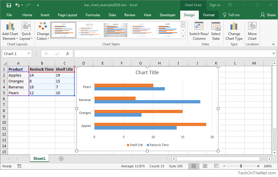
Ms Excel 2016 How To Create A Bar Chart


0 comments: