How To Display Series Name In Excel Chart

Change the Chart Type for the Average series to a Line chart. Select the series Brand A and click Edit.

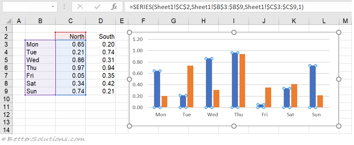
Excel Charts Series Formula

I believe this may resolve your problem.

How to display series name in excel chart. 1 Select cells A2B5. The currently displayed source data is. 3 Select the desired Column type graph.

Edit Series preview pane. Then plot each point as its own series. In the Format Data Series pane under Fill Line tab click Line to display the Line section then check No line option.

Excel then adds these as new columns representing the data series. Just click on the map then choose from the Chart Design or Format tabs in the ribbon. The popup window will show you the chart type for each data series.

Then right click on the line in the chart to select Format Data Series from the context menu. Click anywhere in the chart. Learn how to change the elements of a chart.

Note that the chart does not yet display the 2015 data series. You can change the Chart Title Axis titles of horizontal and vertical axis display values as labels display v. The Edit Series dialog box will pop-up.

Change legend name Change Series Name in Select Data. Click the axis title box on the chart and type the text. This will also expose the map chart specific Series options see below.

Click Select Data button on the Design tab to open the Select Data Source dialog box. Change legend text through Select Data. Right-click anywhere on the chart and click Select Data.

In this example we have a chart that shows 2013 and 2014 quarterly sales data and weve just added a new data series to the worksheet for 2015. SERIES In the case of a bubble chart there is one additional argument. SERIES You can also view the series data using the Select Data dialogReviews.

There are spaces for series name and Y values. Please click to highlight the specified data series you will rename and then click the Edit button. In Excel 2003 choose Options from the Tools menu and skip to 3.

Add titles and series labels Click on the chart to open the Chart Tools contextual tab then edit the Chart title by clicking on the Chart Title textbox. Right click the chart and choose Select Data from the pop-up menu or click Select Data on the ribbon. Then format data labels to display series name for each of.

Since you want the average to show up as a line instead of columns right click on the data series and select Change Series Chart Type. This Excel Trick will help you to DisplayShow Formulas in Excel without any issues. Type the new series label in the Series name.

5 Select Data Labels Outside End was selected below If you dont want the Values as the Labels you can click on. Right click the chart whose data series you will rename and click Select Data from the right-clicking menu. Similarly for more such tips tricks you can follow our Excel Ninja Training and become an expert in Excel.

You can also double-click the chart to launch the Format Object Task Pane which will appear on the right-hand side of the Excel window. 4 Click on the graph to make sure it is selected then select Layout. I have a series of charts I am creating using VBA code below.

Click the File tab and choose Options. Changes over days or weeks andor the order of categories is not important. To edit the series labels follow these steps.

Another convoluted answer which should technically work and is ok for a small number of data points is to plot all your data points as 1 series in order to get your connecting line. Click anywhere within your Excel chart then click the Chart Elements button and check the Axis Titles box. 6 Use a clustered column chart when you want to focus on short term trends ie.

Excel provides a simple way of displaying formulas in the cells instead of the result. 5 Use a clustered column chart when you want to show the maximum and minimum values of each data series you want to compare. My real name is Cory Youll see me all over this thing but I can appreciate a name like Naeblis considering my screenname is what I posted here.

Right hand click on the graph and select Format Data Series then select Data Labels and tick the Show Label option. Now the Select Data Source dialog box comes out. If you want to display the title only for one axis either horizontal or vertical click the arrow next to Axis Titles and clear one of the boxes.

Select Series Data. In the Series name field type Duration or any other name of your choosing. In Excel 2007 click the Office button and then click Excel options.

Fill in entries for series name and Y values and the chart shows two series. Edit Series in Excel. As before click Add and the Edit Series dialog pops up.

Select the series you want to edit then click Edit to open the Edit Series dialog box. I am having trouble changing the names of the series from series 1 and series 2 to Current State and Solution State. Right-click on the series itself and select Format Data Series then click the Data Labels tab and choose the Show Value option.

Alternatively you can place the mouse cursor into this field and click the column header in your spreadsheet the clicked header will be added as the Series name for the Gantt chart.